Throwback Thursday

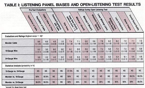
Table I shows the results of the listening panel’s pre-test evaluations of the three cables tested (left part) and their ratings of the cables during the open listening tests (right part), together with a statistical analysis. The ratings in the upper half of the chart are mean scores derived by averaging the questionnaire responses of all the panelists; the numbers shown in parentheses below them are their standard deviations—that is, the statistical spread around each mean score. Thus, the higher the standard deviation, the wider the range of scores.

The lower half of the table indicates whether the differences in the ratings of the three cables are statistically significant. The method of comparison used, the Student’s paired test, estimates the probability that an observed difference in preferences could have occurred by chance. The number given for each comparison in each category or test represents the probability that the difference did not occur by chance alone. Probabilities below 95 percent are considered statistically insignificant and are indicated by “NS.”

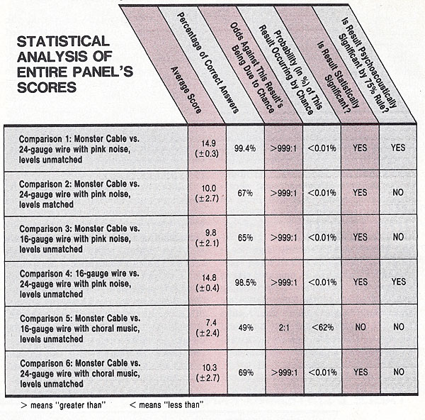
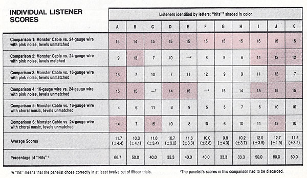
Table II. The two charts on this page show the results of the controlled, double-blind listening comparisons of the three cables. At right are the results for the panel as a whole, together with a statistical analysis of the comparisons. The scores for each member of the panel in each comparison are shown in a separate chart.

The ABX comparator system is statistically similar to flipping a coin and predicting whether it will come up heads or tails. Each of the two results is equally probable, so random predictions are likely to be correct 50 percent of the time. Since each of our comparisons comprised fifteen trials, a listener would have gotten a score of 1.5 if he could hear no differences between the cables and were just guessing. Any score much above 1.5 is thus better than chance and might be significant.

Using published tables of the binomial (“bell-curve”) statistical distribution, we calculated the likelihood of correct scores in each comparison for the entire panel. We found that 91 or more correct answers out of a total of 165 in each comparison gave a probability of 95 percent or more that the results were not due to chance. Results meeting this criterion are thus indicated as statistically significant.

We also used, however, a stronger criterion: psychoacoustical significance. In psychoacoustical testing, it is generally accepted that the threshold at which a phenomenon can be considered definitely audible is when listeners are aware of it at least 75 percent of the time. This is the basis for our definition of a “hit” as at least twelve out of fifteen correct answers. Applied to the scores of the whole panel, this meant that 124 answers out of 165 trials for each comparison had to be correct before we concluded that the differences between the cables were indeed audible.

Results that meet the 75 percent rule are due to more vivid effects than those producing a merely statistically significant result. An additional clue to the magnitude of the differences between the cables tested is the number of listeners who scored a hit in each comparison; the more hits, the more striking were the audible differences.