HOW WE TEST

Measuring Loudspeakers
We publish pseudo-anechoic loudspeaker measurements, another synthetic test that has little to do with real-world conditions. To be anechoic means to be without echoes or sonic reflections. The pseudo comes into play because neither we nor any entity beyond a few speaker manufacturers and research facilities around the world have a true anechoic chamber designed to fully absorb all of a speaker’s reflections. Of course, a real-world listening room is far from reflection free, so you’re unlikely to ever hear (or want to hear) loudspeakers under anechoic conditions. However, this is a generally accepted convention for characterizing loudspeakers. We measure speakers in a very large, open, and high-ceilinged warehouse, so we at least begin in an environment that has few reflective surfaces (and no room boundaries) in the immediate vicinity of the loudspeaker under test. Nonetheless, some clever gating techniques in our LinearX LMS measurement system keep reflected sounds at bay during testing, which eliminates the effect of the surrounding environment.

Below a couple of hundred hertz, we use a technique in which we place the measurement microphone a fraction of an inch from low-frequency sound sources (woofer, port, or passive radiator) to eliminate the possibility of reflections. This close-miking, as we refer to it, is only useful at low frequencies, but it’s a valid technique when implemented appropriately.

To produce a meaningful representation of a loudspeaker’s response over a larger frequency range, we average multiple measurements at a stated distance and at a stated angle. This average of frequencies above a couple of hundred hertz must be combined with low-frequency data derived from close-miking. We measure at a common industry-standard distance of 1 meter, with any included grilles attached on the assumption that most consumers use their gear intact as provided by the manufacturer.

Sensitivity
A loudspeaker’s sensitivity measurement defines, in practical terms, how loud it will play with a standardized input signal as measured from an industry-standard fixed distance. To determine this figure, we measure passive loudspeakers with a drive level of 2.83 volts RMS (equivalent to 1 watt at 8 ohms) using the aforementioned 1-meter microphone distance and pseudo-anechoic (often referred to as “4pi” or “full space”) conditions. The resulting average level from 500 Hz to 2 kHz (an octave on either side of 1 kHz) is noted. This average level is referred to as voltage sensitivity and is expressed in decibels. Loudspeakers with a higher sensitivity can generally be used successfully with a smaller amplifier in a given sized room than their lower-sensitivity counterparts, which will require more amplifier power to produce the same volume level under the same conditions.

Listening Window
Most loudspeakers emit a broad portion of their range of sound from a single face or baffle and are referred to as monopole designs. For these, we start with the listening axis, usually in line with the tweeter unless the manufacturer specifies a different vertical axis. From there, we measure at 15 degrees to the left, to the right, up, and then down from the listening axis, all at a distance of 1 meter. This gives us five response curves, which we average mathematically to produce our version of what is often referred to as a listening-window measurement. The idea here, albeit somewhat oversimplified, is that no one (OK, not many) use a laser pointer to aim each loudspeaker directly at a single listener, so ±15 degrees defines an area, or window, where ears are likely to be situated during the course of listening. Also, it’s expected that any given loudspeaker’s response will be different off axis than on, and this technique takes that into account to some degree in defining an overall response measurement.

We then apply one-third-octave smoothing to this data, which removes many audibly insignificant but visually noticeable narrow-bandwidth wiggles from the curve. This better reveals more of the larger issues likely to affect what you hear. It also leaves us with a graph that presents the important overall trends in the response in a visually communicative manner. This average of all the curves from within this listening window, to our way of thinking, better communicates the nature of a loudspeaker’s performance than a single axial measurement.

Diffuse surround loudspeakers, often referred to as dipole or bipole designs, require a slight variation on the theme above. We still measure at a 1-meter distance on the tweeter or the manufacturer-specified vertical axis. The difference is that we average together measurements from each of the three faces—front, side, and rear—into what we refer to as a three-face averaged response.

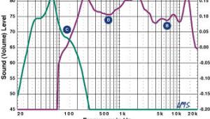
Frequency Response
The graph we publish for each loudspeaker system depicts the response from the industry-standard 20 Hz to 20 kHz. In the text, we call out the –3-dB and –6-dB frequencies, relative to the level in the midband, so the lowest range extension is specified at two levels often quoted in manufacturer brochures. Establishing that midband level from which we measure these roll-off points isn’t straightforward, as there isn’t much of a standard for this specification in the industry. For loudspeakers other than subwoofers, we use the average level from 500 Hz to 2 kHz as the nominal baseline. For example, if the 500-Hz-to-2-kHz average determines that the sensitivity is 90 dB, then we call out the frequency where the level has rolled off to 87 dB as the –3-dB point, the frequency where the level is down to 84 dB as the –6-dB point, etc. If the sensitivity were 86 dB, then the –3-dB point would be the frequency where the level rolls off to 83 dB, and the –6-dB point would be the frequency where the level is down to 80 dB.

For subs, we use the level at 80 Hz. For the sub output of AVRs and surround processors, we use the level at 40 Hz. While 40 Hz would seem to be a logical choice for subwoofers, too, we cover an amazingly broad range of products, and not every sub we measure is flat down to 40 Hz.

We call out the listening window plus-or-minus tolerance, which is intended to give you insight into the smoothness of the response over the majority of the operating range. We chose a range of 200 Hz to 10 kHz, as this is within almost every loudspeaker’s passband, covering the astounding range of models we measure. For example, many small satellite loudspeakers are expected to be bass limited –6 dB at 100 Hz or higher, so if our listening-window range were specified to 100 Hz or lower, often the bottom number would reflect only the loudspeaker’s expected rolloff, not point a finger at a potential problem elsewhere (that is, higher up) in the response.

So what should this response curve look like for general-purpose loudspeakers? A consensus may be difficult to come by, but as a rough rule of thumb, a smooth, fairly flat graph line is the desired result. If there are deviations, dips below the median are generally preferable to peaks that rise above it, and aberrations over a narrow range of frequencies are likely to have less of an impact than broad ones. Observable tilt from one end of the graph to the other, either incline or decline, should be minimal as well.

Impedance
Finally, we measure the electrical impedance of passive loudspeakers from 20 Hz to 20 kHz. As many serious audiophiles know, a speaker’s rated impedance is nominal—essentially an approximation of the actual load. But true impedance varies with frequency. We note the minimum impedance in ohms that could be presented to the amplifier between 20 Hz and 20 kHz, the largest phase variance in degrees, and state the frequencies at which each occurs. The phase angle tells us how much the amplifier will have to struggle with providing voltage versus current to the speaker as the load demands it. Values beyond ±60 degrees will usually make for a hotter-running amplifier. This information, along with sensitivity, is most helpful when used as a tool to aid in matching an appropriate amplifier to the demands of a specific loudspeaker model.

Conclusion
While these thoughtfully derived and meticulously executed audio tests provide a window into a component’s or speaker’s engineering ethos and electrical performance—and help us identify issues that may manifest sonically—they can’t tell the whole story. In the end, it’s the sound that counts, and for the final word on that, we rely at Home Theater on the observations and judgments of our expert reviewers. Unlike a microphone or an audio analyzer, reviewers bring their prior experience, biases, personal tastes in music and movie content, and even their own physiology of hearing to the process of evaluating a product. Hopefully, with the insights you’ve gained here, you can now read through our concise Audio Measurements Box and find comfort in the one constant we can provide you across all audio reviewers and reviews.